(Click picture to enlarge.)

Readers may have seen two charts that are part of a column by David Wessel published last week. For five European countries, they compare actual interest rates with those prescribed by a standard policy rule. Wessel’s charts provide some interesting evidence that European Central Bank monetary policy has been either too loose or too tight most of the time for several currently ailing European economies, given these countries’ inflation rates and gaps between actual and potential output.  Wessel’s charts support the article’s theme, which is that severe economic problems in some Eurozone countries result in part from the “one-size-fits-all” interest rate policies of the ECB.

Along the same lines, at the top of this entry is a chart of short-term “real interest rates” faced by business borrowers who use overdraft loans in a group of European countries, which are mostly members of the euro area. I have used data on interest rates for this common type of loan, adjusting each month’s observation to reflect the same month’s measured consumer price inflation, so that the resulting “real rates” take into account inflation’s effects on the burden of loan payments. Inflation is helpful to debtors because it has the effect of reducing the amount of goods and services represented by each dollar owed under the terms of a loan. Of course, I have used only one of many possible methods that one could employ to approximate real interest rates.  Moreover, to construct a true real interest rate data series, one would need to know borrowers’ forecasts of the inflation rate, which is an impossible requirement in most circumstances. Hence, these series and others like them usually need to be taken with a grain of salt.

As theory would have it, real interest rates in different countries tend over the long run to converge on a common value, a result known as “real interest rate parity.” This convergence is assured only under certain exacting conditions that are clearly not met in the case of the numbers depicted in the chart. Nonetheless, the degree to which the rates differ may provide another indication of the disparities in credit costs that are imposed by a unified central banking system. Moreover, the chart shows that some of the countries now experiencing fiscal crises have been suffering the effects of particularly tight credit conditions. For example, Greece’s real interest rate was 20.49 percent in January, as indicated next to the green line representing the Greek data. Real rates for Ireland and Portugal, two other countries whose governments’ financial problems have recently been in the news, are also shown in the figure.

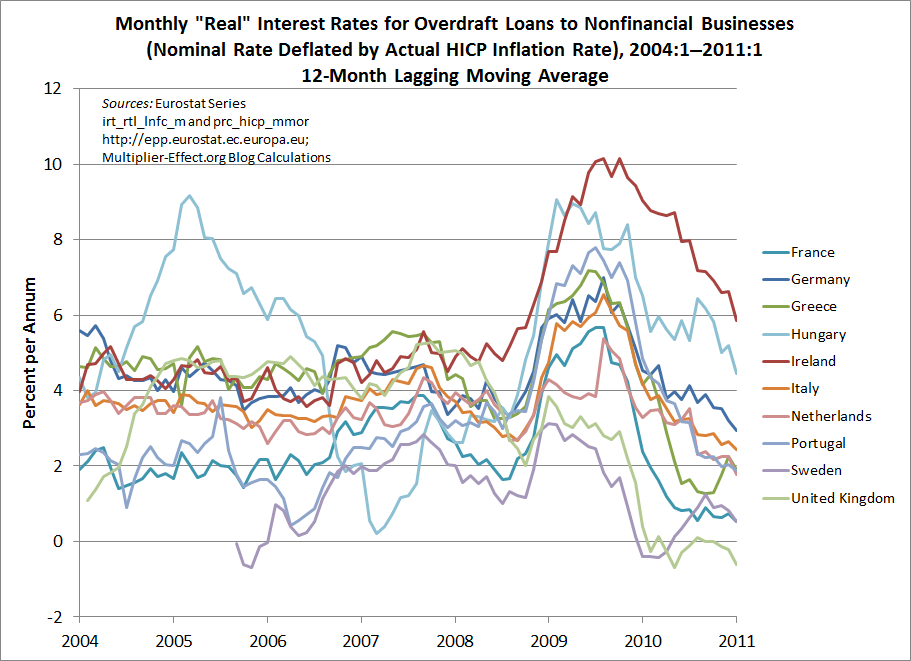
My next chart shows lines for all of the aforementioned countries, plus 7 others, containing points that are constructed by averaging the last 12 months’ observations from the first chart.  This removes most of the effects of regular seasonal patterns and helps to highlight longer-run trends, which would otherwise be obscured by the extreme volatility of these series. As a result, we are able to include data for 10 European nations in this figure.

(Click picture to enlarge.)

The data underlying the figures are harmonized European statistics, which are meant to be somewhat comparable across national boundaries. Nevertheless, the ten series in the figure seem to show no signs of converging, though their movements appear to be highly correlated over the past three years. According to the averaged data, Irish real interest rates have been the highest among the 10 European economies represented in the graph since approximately spring 2009. In January, the unaveraged real rate in Ireland exceeded 9 percent.

Like Wessel’s diagrams, the ones above show that despite centralized interest-rate setting, one measure of the tightness of policy for actual retail borrowers varies greatly across eurozone economies.

Notes:

continue reading…

Some more thoughts on the federal debt, which I blogged about last week: First, at Barry Ritholtz’s blog, there are some other interesting figures: one portraying the gross federal debt in three different ways and another breaking the gross debt down by holder. Ritholtz’s figures use data from the U.S. Treasury Department. Note that the gross debt, which stands at a little over $14 trillion, includes around $3 trillion in securities held by the Social Security and Medicare trust funds. (See Trustees’ report.) These securities are not treated as federal liabilities in flow-of-funds data, the main source for the figures in my earlier post. This difference between net and gross numbers accounts for most of the apparent gap between the figures reported in Ritholtz’s blog and those reported here. Like the Federal Reserve’s portfolio of Treasury securities, the securities owned by the trust funds are essentially both assets and liabilities for the broader federal sector, and for macroeconomic purposes, it is best to net them out in my opinion. This leaves well below $10 trillion in federal debt to the public, according to both flow-of-funds data and the Treasury Department website. Regardless of the exact size of the federal debt, which is not crucial, the point to note right now about the deficit issue is that the economy does not appear to be showing signs of excessive government borrowing. We at the Levy Institute will be writing more about this in the near future.

Along these lines, it was good to see Bill Mitchell’s recent article on the deficit in The Nation. Many of the points raised by Mitchell are crucial to the deficit debate and well expressed in the article.

(Click on graph to enlarge.)

Some interesting information on the federal government’s balance sheet can be gleaned from the fourth-quarter flow-of-funds report, which was released by the Federal Reserve Board on the 10th of this month. The total amount of all federal liabilities, as reported by the Fed last week, is shown as the sum of the red and blue areas in the figure above. The blue portion of the graph represents net liabilities owed by the federal government to the Federal Reserve System, while the red portion shows the rest of the federal government’s liabilities. The blue portion is best netted out of the total debt when one is calculating a figure to be used for policy purposes, as it essentially represents a sum of money that one part of the federal government owes to another. (The Fed describes itself in its educational literature as “independent within the government,” though it is shown in flow-of-funds reports as a separate entity with a separate balance sheet from that of the federal government.)

As noted in the figure above, total federal liabilities, according to the new data, rose in the fourth quarter of 2010 to 75.0 percent of seasonally adjusted U.S. GDP from 72.6 percent the previous quarter. Of this 2.4 percentage-point increase, 1.6 percentage points were accounted for by an increase in net Fed holdings of federal government liabilities, while all other entities increased their combined holdings of these liabilities by only about nine-tenths of a percentage point. Hence, ignoring the more-of-less irrelevant holdings of the Fed, the federal debt stood at approximately 65.5 percent of GDP as of the end of last quarter.

When the Fed purchases federal government liabilities using its open market account, it is swapping money for debt securities, so that economic sectors other than the Fed and the federal government wind up holding more U.S. currency and/or reserve deposits and fewer interest-bearing U.S. liabilities than before. This helps the Fed keep interest rates lower than they otherwise would have been as the total debt rises. Dimitri Papadimitriou and I discuss the increased use of this “financing” strategy in a recent working paper.

A couple of minor technical points: These figures are approximate and do add up in some cases because of rounding. Also, the Fed liabilities data are not seasonally adjusted, though, as noted above, I have divided them by seasonally adjusted GDP figures from the FRED database at the St. Louis Fed website.

Revised to improve clarity by G. Hannsgen on March 17, 2011 at approximately 8:20 am. Specifically, I have clarified the point that the blue portion of the figure, representing federal government liabilities to the Fed, is a net amount. In other words, it shows the amount of federal liabilities to the Federal Reserve System minus the amount of liabilities that the Fed owes to the federal government, all divided by GDP and expressed in percentage terms. Some discussion of this point might have been helpful. To wit: most of the federal government’s liabilities to the Fed are Treasury securities; an example of the opposite variety would be one or another of the several “bank accounts” that the government holds at its central bank. To determine how much the federal government owes the Fed, one must subtract the balance in these bank accounts and the like from the government’s gross liabilities to the Fed. It is only such net amounts that are shown in the blue portion of the figure above. Those figures are in turn subtracted from total federal liabilities as reported in quarterly flow-of-funds data to yield approximations of the quarterly “true” federal debt, which are, of course, depicted by the red area in the picture.

(Click figure to enlarge.)

Two Fridays ago, I blogged about some newly released Bureau of Labor Statistics (BLS) data from a monthly household survey. I was surprised later to see that Multiplier Effect was one of only a handful of websites to mention that non-seasonally adjusted data showed vastly different and perhaps more disturbing results than the widely reported deseasonalized numbers: a flat unemployment rate, a sharp fall in employment, and a rise in the number of people unemployed. All of the numbers I discussed were based on traditional concepts of unemployment, which have been familiar to newspaper readers for decades.

It is important to put such survey results in context, and I have now had time to finish putting together some further information on the effects of seasonal adjustment on the numbers released early this month. While the standard version of the unemployment rate is widely reported and debated, it does not include potential workers who are not considered to be in the labor force because they have not recently been looking for work. If the labor market were stronger, most of these individuals would almost certainly return to the workforce and find work. Hence, it is interesting to look at a broader measure of unemployment that includes at least some of those out of workforce who want to work, but have not recently been searching for a job.

One such statistic is the BLS’s own U-4 measure of “labor underutilization,” which includes those deemed to be “discouraged workers,” in addition to the unemployed. The seasonally adjusted version of U-4 dropped from 10.2 percent in December to 9.6 percent in January. In contrast, the non-seasonally adjusted version of this index rose from 9.9 percent to 10.4 percent, according to the BLS. Hence, the story we have told in blog entries over the last two weeks also seems to have some implications for a more comprehensive measure of the human cost of weakness in the labor market.

The simple methodology that I used in my most recent post on the BLS report to calculate the impact of seasonal adjustment on the month-to-month change in the unemployment rate can be extended to a broader but unofficial index. This time, my answer will be somewhat less exact, because we do not have complete information about the potential impact of the 2011 adjustments to BLS population estimates on my new calculations .

Using data from Table A-1 of the BLS news release, as well as partial information on the effects of population adjustments on the January data from Table C of the release summary, we can find the contribution of seasonal adjustment to the apparent change in the following seasonally adjusted makeshift unemployment index:

number unemployed + number out of the labor force who want to work

divided by

labor force + number out of the labor force who want to work

The BLS does not separately report this statistic to our knowledge, but it is similar in spirit to several other alternative gauges of labor underutilization reported in Table A-15 of the employment report. Hence, we report our findings with the caveat that the BLS certainly might not endorse the use of this improvised measure.

What we find is interesting: seasonally adjusted BLS numbers from table A-1 imply that our broad unemployment index dropped from 13.0 percent in December to 12.7 percent last month. These are large numbers indeed. However, removing the effects of seasonal adjustment on the underlying raw numbers, the broad index probably would have risen by at least .9 percent, from 13.0 percent in December to between 13.9 and 14.0 percent. Hence, using a similar methodology to last week’s post, one finds that the effect of seasonal adjustment on the change in the broad unemployment measure is even greater than the corresponding effect on the change in the usual measure.

By the way, other data in the recent government report suggest that this difference between seasonally adjusted and non-seasonally unadjusted figures can largely be accounted for by temporary layoffs whose impact on the data was removed by adjustment procedures.  In other words, many workers were laid off last month, but were not counted in the most widely reported January unemployment figures, because large numbers of layoffs are not unusual for that time of year.

In fact, the historical record shows that the effects of BLS seasonal adjustment procedures are often especially large for the January release, resulting in substantial downward statistical adjustments to the recorded change in the unemployment rate from the previous December. This effect is not often noted in the media, though non-seasonally adjusted BLS figures are made available in the same report as the headline unemployment rate. The blog seekingalpha wrote about this phenomenon last winter. The figure at the top of this post is similar to a graphic appearing in that blog entry.

Edited slightly for clarity and readability Feb. 16 at 12:11 pm.

The White House remedies for the mortgage meltdown have now been presented. Congress will debate the life extension, death, or rebirth of federal mortgage entities Fannie Mae and Freddie Mac during the coming weeks. When the noise has died down, don’t expect substantial change. But those who hope for genuine financial reform should, nonetheless, listen carefully not only to what Washington says, but to whom it says it. Will the new guidelines call on traditional home-loan bankers to make traditional loans? Or will we hear a shout-out to the investment bankers/mortgage traders who designed the mess? In any new financial structure for home loans, the single most important issue will be the ratio of debt to assets that the government will expect lenders to show. During the real estate boom, lenders were willing—and able—to provide mortgage brokers with financing for 100 percent or more of the value of a property with the expectation that real estate prices would rise. We witnessed the triumph of the trader over the banker: Profit relied on the sale or refinancing of the asset. For a mortgage originator or securitizer with no plans to hold on to the mortgage, what really matters has been the ability to place it, not the depth of the underwriting or the long-term financial prospects of the home resident. A traditional banker, on the other hand, might feel safe with a capital leverage ratio of twelve to one, with careful underwriting to ensure that the borrower would be able to make payments. With equity at risk, something close to that level of underwriting would be essential. The trader-think model virtually eliminated mortgage underwriting. What we saw instead has been succinctly described by L. Randall Wray in a Levy Institute Brief (http://www.levyinstitute.org/publications/?docid=1301): “Property valuation by assessors who were paid to overvalue real estate, credit ratings agencies who were paid to overrate securities, accountants who were paid to ignore problems, and monoline insurers whose promises were not backed by sufficient loss reserves…” Much of the activity didn’t even appear on the balance sheets. Mortgage brokers arranged for finance, investment banks packaged the securities, and the shadow banks — the managed money — held the securities. The debt to assets ratios for mortgages climbed. Investment bankers consolidated their liabilities into a single financial market that could have been called the Mortgages & More Shoppe. Mortgage-backed securities were included with commercial banking, and with other financial services where acceptable capital leverage ratios are much higher than for traditional home loans. (For money managers, capital leverage ratios can be 30 to 1 and up to several hundred, with even higher unknown and unquantifiable risk exposures.) Income flows took a backseat. Except for the home resident, that is. Because ultimately, all of these financial instruments came to rest on the shoulders of some homeowner trying to service her mortgage out of annual income flows which boiled down to, on average, five dollars worth of debt and only one dollar of income to service it. “In an ideal world,” Wray added, “A lot of the debts will cancel, the homeowner will not lose her job, and the FIRE (finance, insurance, and real estate) sector can continue to force 40 percent of… profits in its direction. But that is not the world in which we live. In our little slice of the blue planet, the homeowner missed some payments, the securities issued against her mortgage got downgraded, the monoline insurers went bust, the credit default swaps went bad when AIG failed, the economy slowed, the homeowner lost her job and then her house, real estate prices collapsed, and, in spite of its best efforts to save [the system], the federal government has not yet found a way out of the morass.” Whatever the fate of Fannie Mae and Freddie Mac, the coming federal recommendations need to lift underwriting standards up from that morass and back onto solid ground. According to January’s Financial Crisis Inquiry Commission report, about 13 million US homes have already or will soon face foreclosure. The investment bank traders who securitized those mortgages, with a few notable exceptions, have overwhelmingly escaped such suffering. Financial reform should change that equation by demanding a traditional, appropriate ratio of assets to debts in the real estate markets.

In Friday’s post, I pointed out that unemployment and employment numbers announced by the BLS had apparently been changed greatly by the process of adjusting for typical seasonal changes. These adjustments are meant to account, for example, for the fact that retail business is generally stronger than usual during the holiday season at the end of each year. Friday’s widely reported unemployment drop to 9.0 percent in January from 9.4 percent the previous month was a figure that had been seasonally adjusted by the BLS to remove such normal seasonal effects. Also reported by the BLS Friday in the same set of documents were non-seasonally adjusted numbers that showed an increase in unemployment from 9.1 percent in December 2010 to 9.8 percent in January 2011. Few internet news outlets seem to have reported these latter percentages or the underlying raw numbers used to calculate them. On the other hand, many blogs and other news sources mentioned that adjustments had been made to the official numbers to reflect improved estimates of population growth from recent surveys, resulting in a problem with comparing January’s numbers with December’s. Friday morning’s blog post contained a qualifying statement to the effect that these population-related statistical adjustments had probably affected the un-seasonally adjusted numbers that I reported in the same post. Here is what I have been able to figure out about the importance of these two factors in creating such a large difference between the seasonally adjusted and non-seasonally adjusted one-month changes in the unemployment rates reported by the BLS.

The seasonally adjusted drop in number of unemployed people was -622,000, according to the BLS figures reported Friday. Table C in the accompanying news release estimated that annual changes in population estimates made by the BLS each January had this year magnified the reduction in unemployment from December to January by +32,000 individuals, leaving a true drop of perhaps −590,000, once one removed the effect of the population adjustments. On the other hand, non-seasonally adjusted figures from the same economic news release (Table A-1) showed an increase in the number of unemployed people of +40,000. Hence, one can deduce that, at least to a rough approximation, seasonal adjustment resulted in a much larger swing than population-related adjustments in figures reported in the headlines yesterday. Namely, about 630,000 more people were unemployed last month, once one puts back in the effects of typical seasonal changes in unemployment, as estimated by the BLS, resulting in a swing in the estimated figures of approximately +.4 percent of the labor force. In other words, the reported reduction in the unemployment rate from 9.4 percent to 9.0 percent in January derived from household survey data can be accounted for almost entirely by seasonal adjustments applied by the BLS.

Minor corrections for readability made to the post above approximately 2:00 pm, February 6 by G. Hannsgen

A note on the unemployment figures released earlier this morning by the Bureau of Labor Statistics (BLS), reporting the results of a January survey of U.S. households: The seasonally adjusted unemployment rate fell from 9.4 percent in December to 9.0 percent last month, a healthy improvement. On the other hand, before seasonal adjustment, the unemployment rate rose from 9.1 percent in December to 9.8 percent in January. Raw data that are not seasonally adjusted show that the number of unemployed Americans rose by 940,000, while the number employed fell by 1,560,000. New adjustments for population changes, introduced by the BLS this month, affected these numbers by an amount that is possibly very large and that is not yet known to me. This latter problem probably affects raw numbers more than the overall unemployment rate. The seasonally unadjusted numbers used in this blog post can be found in table A-1 of the recent economic news release from the BLS.

In December, the Levy Institute issued a working paper that asked how the economy might be affected by the seemingly unusual fiscal and monetary policies implemented by the Fed and other central banks since 2008. The authors, Dimitri Papadimitriou and I, used a phrase that is not often spoken in this era by governments and central banks around the world: “monetizing the deficit.” This phrase traditionally describes the practice of financing a government deficit with money that is “printed” rather than borrowed or raised by taxation. We feel perhaps a little more comfortable with our use of these words in light of a recent blog entry on the Financial Times website Alphaville. The blog reports that the Fed has come close to running out of securities to buy in the markets for certain types of government bonds, having bought so many of them already. Hence, it is increasingly resorting to the purchase of recently issued bonds and notes, which it had apparently sought to avoid. This development makes the link between deficit spending and monetary policy initiatives such as the current round of “quantitative easing” in a monetary system like ours easier to grasp. If the Fed buys a Treasury security almost immediately after it is issued, there is less reason than ever to think of the financing process as anything other than the use of the Federal Reserve’s “printing press” to pay for government operations–an essential use of “monetization” to stimulate the economy and avoid drastic fiscal measures during a time of weak tax revenues. Some worry still, but this practice has been used many times by numerous governments around the world and seems unusual only in light of common but unrealistic beliefs about monetary systems and how they normally work. Hence, those in Congress should not give credence to arguments that it is necessary to eliminate entire government programs or freeze major parts of the federal budget in order to restore some fanciful state of budgetary normalcy.

February 10 addendum on recent news: A short and interesting article on the implementation of quantitative easing policies was posted very recently on the New York Fed’s website. The article mentions changes in the composition of the Fed’s asset purchases, including the recent increase in purchases of newer issues that was reported in the Alphaville blog entry linked to above.  On the other hand, the new piece, based on a speech by a Fed official, finds no evidence that the Fed’s purchases have caused “significant market strains.” The article covers some other important issues associated with the recent policy actions involving long-maturity securities and might be interesting to people wanting detailed information about these topics.

Reading the back and forth between Brad deLong and David Leonhardt over the structural versus cyclical nature of unemployment during the Great Recession, a question nagged at me, spurred by this quote from Leonhardt:

The data that the Bureau of Labor Statistics released on Thursday gives me a chance to explain why I disagree. In short, the relative performance of more educated and less educated workers over the last few years has not been the typical pattern for a recession. Less educated workers, by many measures, are faring worse than they ever have.

The ratio of the typical four-year college graduate’s pay to a typical high-school graduate’s pay hit a record in 2010 — 1.56. Since 2007, the inflation-adjusted median weekly pay of college graduates has risen 1.6 percent. The inflation-adjusted pay of every other educational group — high school dropouts, high school graduates and people who attended college but did not get a four-year degree — has fallen since 2007. The same is true over the last decade; amazingly, only college graduates have received a raise.

continue reading…

U.S. Long-Term Government Bond Interest Rates, 1925-2010

Last summer, this blogger posted a graph showing the path followed by U.S. long-term interest rates since 1925.  There has been some interest in a new and updated graph, especially in light of concerns that bond markets might soon demand higher yields as the economy expanded. One appears above. Reasons for apprehension about a possible jump in yields vary and include large federal deficits, which increase the amount of bonds that must be absorbed by the market, as well as concerns about a possible resurgence of inflation driven by quantitative easing (QE) and a near-zero Federal Funds rate.  The Financial Times [homepage link] and some other newspapers have been reporting recently on a perhaps greater threat to price stability worldwide: a continuing run-up in the prices of some key agricultural commodities, brought about mostly by factors other than macroeconomic policy.  There has been some discussion of rising yields for long-term government bonds, but the long-term perspective offered by the figure above shows that interest rates remain very low by historical standards, at least for now.

Moreover, real yields on federal inflation-indexed securities remain quite low indeed, and in some cases negative, as shown, for example, by the green line in the figure below. Broadly speaking, such yields are what markets expect certain inflation-protected bonds to yield in addition to compensation for inflation.  Hence, they can be viewed as indicators of the costs of borrowing after expected inflation is taken into account. These costs have apparently been trending downward since 2008. (Some related but different interest rate series remain in positive territory, including for example one type of ten-year inflation-indexed bond issued early last year, which is yielding a little over .8 percent. By the way, the red line in the graph below shows only the most recent data points from the figure at the top of this post. This  longer-term nominal rate is not comparable to the inflation-indexed series depicted by the other line.)  These data show that recent Fed efforts to ease the terms on which money can be borrowed in a time of large deficits have continued to prove efficacious in a way that many economists find puzzling, though it is unlikely that these monetary policy actions alone will have a large impact on the rate of economic growth.

Nominal Interest Rate (shown in red) and "Real Rate" (shown in green)